Probabilistic Generative Model

The generative approach to classification (PGM), works by:

1. Estimate the class-conditional probabilities, $p(\mathbf{x}|C_j)$ - which can be used to generate new data points, hence the name ‘generative model’
2. Calculate the posterior probability using Bayes Theorem: $P(C_j|\mathbf{x})\propto p(\mathbf{x}|C_j)\cdot P(C_j)$

Key Steps

To solve for the posterior probabilities $P(C_j|\mathbf{x})$ via PGM, we follow the key steps:

1. Expand the posterior using logistic/softmax functions
2. Determine form of arguments to the softmax function (with model assumptions)
3. Estimate parameters for the resulting form

Expanding the Posterior

Two Class Case

Let us consider the key steps for the simple case of two classes.

$$P(C_2)=1-P(C_1)$$

We know the equation for joint probability to be:

$$p(x,y)=p(x|y)\cdot p(y)$$

We also know the sum rule (marginalisation):

$$p(x)=\sum _{y}p(x,y)$$

And the product rule

$$p(x,y)=p(y|x)\cdot p(x)$$

With this, we can expand the posterior:

NOTE: the lecturer mentioned this being in the A1 likely!

$$\begin{array}{rl}P(C_1|\mathbf{x})& =\frac{P(C_1,\mathbf{x})}{P(\mathbf{x})}\text{ (from the definition of joint probability)}\\ & =\frac{P(\mathbf{x}|C_1)P(C_1)}{P(\mathbf{x})}\text{ (from the product rule)}\\ & =\frac{P(\mathbf{x}|C_1)P(C_1)}{P(\mathbf{x},C_1)+P(\mathbf{x},C_2)}\text{ (from the sum rule)}\\ & =\frac{P(\mathbf{x}|C_1)P(C_1)}{P(\mathbf{x}|C_1)P(C_1)+P(\mathbf{x}|C_2)P(C_2)}\text{ (from the product rule)}\\ & \text{We’re now going to coerce this into a logistic form}\\ & =\frac{1}{1+\frac{P(\mathbf{x}|C_2)P(C_2)}{P(\mathbf{x}|C_1)P(C_1)}}\text{ (divide by numerator)}\\ & =\frac{1}{1+e^{\ln \frac{P(\mathbf{x}|C_2)P(C_2)}{P(\mathbf{x}|C_1)P(C_1)}}}\text{ (turn to exponential)}\\ & =\frac{1}{1+e^{-\ln \frac{P(\mathbf{x}|C_1)P(C_1)}{P(\mathbf{x}|C_2)P(C_2)}}}\text{ (flip the fraction)}\\ & \text{Now, let us define }a\text{ to be the ln function}\\ & =\frac{1}{1+e^{-a(\mathbf{x})}}\\ & \text{We can now notice that this is the sigmoid function}\\ & =\sigma (a(\mathbf{x}))\end{array}$$

Let’s have a closer look at the implications of the definition of $a(\mathbf{x})$:

Some background, the odds of an event $E$ is defined as:

$$\text{odds}(E)=\frac{P(E)}{1-P(E)}$$

We can use this to say the prior odds (odds without an observation) for class $C_1$ is:

$$\text{odds}(C_1)=\frac{P(C_1)}{1-P(C_1)}=\frac{P(C_1)}{P(C_2)}$$

Similarly, the posterior odds (odds given an observation) is:

$$\begin{array}{rl}\text{odds}(C_1|\mathbf{x})& =\frac{P(C_1|\mathbf{x})}{P(C_2|\mathbf{x})}\\ & =\frac{P(\mathbf{x},C_1)P(C_1)}{P(\mathbf{x},C_2)P(C_2)}\text{ (product rule)}\end{array}$$

Look familiar? This means that $a$ is the log-posterior odds of $C_1|\mathbf{x}$

$$a(\mathbf{x})=\ln \text{odds}(C_1|\mathbf{x})=\ln \frac{P(\mathbf{x}|C_1)P(C_1)}{P(\mathbf{x}|C_2)P(C_2)}$$

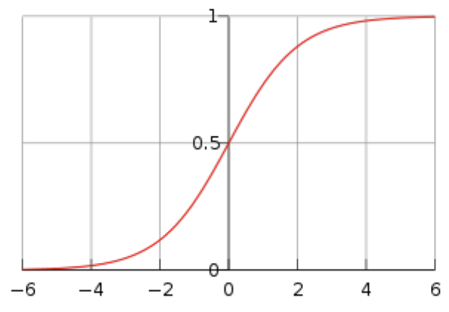
Therefore, the posterior probability $P(C_1|\mathbf{x})$ is the logistic function (sigmoid) evaluated at the log-posterior odds of $C_1|\mathbf{x}$

What does this mean?!

The logistic sigmoid function (as above), takes the log-posterior odds $a(\mathbf{x})$ and maps it to a value between 0 and 1, thereby assigning a posterior probability to $\mathbf{x}$

$\mathbf{x}$ belongs to class $C_1$ if $\text{odds}>1$, otherwise $C_2$

k-Class Case

We can expand the two class case above to a general $k$-class case:

$$\begin{array}{rl}P(C_n|\mathbf{x})& =\frac{P(\mathbf{x}|C_n)P(C_n)}{{\sum }_{j=1}^{k}P(\mathbf{x}|C_j)P(C_j)}\\ & =\frac{\text{exp}(a_n(\mathbf{x}))}{{\sum }_{j=1}^k\text{exp}(a_j(\mathbf{x}))}\end{array}$$

This is the basis of the Softmax Function

Notice that the $a_n(\mathbf{x})$ function is not the log-posterior odds as before

$$a_n(\mathbf{x})=\ln (P(\mathbf{x}|C_n)P(C_n))=\ln P(\mathbf{x}|C_n)+\ln P(C_j)$$

Also note, the total posterior probability must add to 1

$$\sum _{j=1}^{k}P(C_j|\mathbf{x})=1$$

What’s next?

PGM requires two more things:

• Prior class probabilities $P(C_j)$
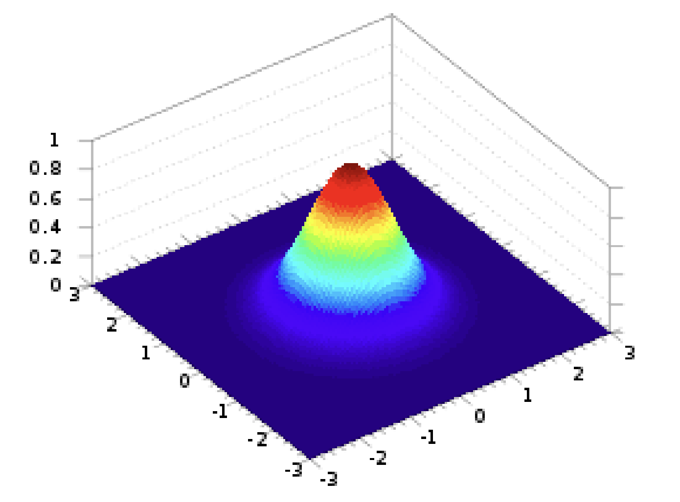
• Class conditional densities $p(\mathbf{x}|C_j)$ which we’ll assume is Gaussian in this course (GaussianNB in scikit-learn)

Gaussian Class-Conditional PDFs

$$p(x|C_j)=\frac{1}{\sqrt{|2\pi {\Sigma }_j|}}\exp \left(-\frac{1}{2}(\mathbf{x}-{\mu }_j{)}^T{\Sigma }_j^{-1}(\mathbf{x}-{\mu }_j)\right)$$

Let’s break this down:

• $|2\pi {\Sigma }_j|$ is a determinant
• ${\mu }_j$ is the mean vector for each class $C_j$
• ${\Sigma }_j$ is the class covariance matrix

We’re going to assume that the class covariance matrices are the same across all classes

$${\Sigma }_j={\Sigma }_i=\Sigma$$

What’s our Log-Posterior Odds?

Two Class Case

Since we now know the class conditional PDFs, we can calculate the log-posterior odds for the two class case as we did before, assuming shared $\Sigma$:

$$\begin{array}{rl}a(\mathbf{x})& =\ln \frac{P(\mathbf{x}|C_1)P(C_1)}{P(\mathbf{x}|C_2)P(C_2)}\\ & =\ln P(\mathbf{x}|C_1)-\ln P(\mathbf{x}|C_2)+\ln \frac{P(C_1)}{P(C_2)}\\ & =-\frac{1}{2}(\mathbf{x}-{\mu }_1{)}^T{\Sigma }^{-1}(\mathbf{x}-{\mu }_1)+\frac{1}{2}(\mathbf{x}-{\mu }_2{)}^T{\Sigma }^{-1}(\mathbf{x}-{\mu }_2)+\ln \frac{P(C_1)}{P(C_2)}\\ & =-\frac{1}{2}\left[{\mathbf{x}}^T{\Sigma }^{-1}\mathbf{x}-2{\mu }_1^T{\Sigma }^{-1}\mathbf{x}+{\mu }_1^T{\Sigma }^{-1}{\mu }_1\right]\\ & +\frac{1}{2}\left[{\mathbf{x}}^T{\Sigma }^{-1}\mathbf{x}-2{\mu }_2^T{\Sigma }^{-1}\mathbf{x}+{\mu }_2^T{\Sigma }^{-1}{\mu }_2\right]+\ln \frac{P(C_1)}{P(C_2)}\\ & ={\mu }_1^T{\Sigma }^{-1}\mathbf{x}-\frac{1}{2}{\mu }_1^T{\Sigma }^{-1}{\mu }_1-{\mu }_2^T{\Sigma }^{-1}\mathbf{x}+\frac{1}{2}{\mu }_2^T{\Sigma }^{-1}{\mu }_2+\ln \frac{P(C_1)}{P(C_2)}\\ & =({\mu }_1-{\mu }_2{)}^T{\Sigma }^{-1}\mathbf{x}+\left[\frac{1}{2}\left({\mu }_2^T{\Sigma }^{-1}{\mu }_2-{\mu }_1^T{\Sigma }^{-1}{\mu }_1\right)+\ln \frac{P(C_1)}{P(C_2)}\right]\end{array}$$

Wow! If we make $\Sigma$ shared, the quadratic terms (${\mathbf{x}}^T{\Sigma }^{-1}\mathbf{x}$) cancels out, resulting in a linear classifier. Let’s define some terms to make it more obvious:

• ${\mathbf{w}}^T=({\mu }_1-{\mu }_2{)}^T{\Sigma }^{-1}\Rightarrow \mathbf{w}={\Sigma }^{-1}({\mu }_1-{\mu }_2)$
  • _we can do $({\Sigma }^{-1}{)}^T={\Sigma }^{-1}$ _since the covariance matrix is symmetrical _
• $w_0=\frac{1}{2}\left({\mu }_2^T{\Sigma }^{-1}{\mu }_2-{\mu }_1^T{\Sigma }^{-1}{\mu }_1\right)+\ln \frac{P(C_1)}{P(C_2)}$
  • Which is the bias term (constant) and contains the prior probabilities

Making the log-posterior probability simplified to:

$$a(\mathbf{x})={\mathbf{w}}^T\mathbf{x}+w_0$$

With the shared $\Sigma$, we have a diagonal matrix, therefore containing $\frac{d\cdot (d+1)}{2}$ parameters. Each ${\mu }_i$ also contains $d$ parameters. Therefore, the total amount of parameters required for the two class generative classifier is:

$$2d+\frac{d\cdot (d+1)}{2}\text{ from }{\mu }_1,{\mu }_2\text{ and }\Sigma$$

Where’s the decision boundary?

Where the probability of both classes are the same, i.e. they equal 0.5.

$$\begin{array}{rl}P(C_1|\mathbf{x})& =P(C_2|\mathbf{x})=1-P(C_1|\mathbf{x})\\ & =\frac{1}{2}\\ \sigma ({\mathbf{w}}^T\mathbf{x}+w_0)& =\frac{1}{2}\\ \therefore {\mathbf{w}}^T\mathbf{x}+w_0& =0\text{ (sigmoid is 0.5 at 0)}\end{array}$$

k-Class Case

Similar to above, we can find:

$$\begin{array}{rl}P(C_j|\mathbf{x})& =\frac{\text{exp}(a_n(\mathbf{x}))}{{\sum }_{j=1}^k\text{exp}(a_j(\mathbf{x}))}\\ a_j& ={\mathbf{w}}_j^T\mathbf{x}+w_{j0}\\ {\mathbf{w}}_j& ={\Sigma }^{-1}{\mu }_j\\ w_{j0}& =\frac{1}{2}{\mu }_j^T{\Sigma }^{-1}{\mu }_j+\ln P(C_j)\end{array}$$

Parameter Estimation

To find the parameters for the class conditional densities and the prior probabilities we need a fully observed dataset, this means observations along with their class labels.

Maximum Likelihood Estimation (MLE)

We can determine the means and covariance matrix for each class using the usual methods:

Means:

$${\mu }_j=\frac{1}{N_j}\sum _{\{i:y_i\in C_j\}}{\mathbf{x}}_i$$

With $N_j$ being the amount of observations in class $C_j$

Covariances:

$${\Sigma }_j=\frac{1}{N_j}\sum _{\{i:y_i\in C_j\}}({\mathbf{x}}_i-{\mu }_j)({\mathbf{x}}_i-{\mu }_j{)}^T$$

From maximum likelihood, we can find the prior probabilities as:

$$P(C_j)=\frac{N_j}{N}$$

The Flaws of MLE

The MLE approach is expensive to compute. With $d$ input dimensions and $k$ classes:

• each class has a mean with $d$ parameters
• each class has a symmetrical covariance matrix containing $\frac{d\cdot (d+1)}{2}$ parameters

This results in a parameter count of

$$k\left[d+\frac{d\cdot (d+1)}{2}\right]=\frac{k\cdot d\cdot (d+3)}{2}$$

If we share the covariance matrix, this reduces to:

$$kd+\frac{d\cdot (d+1)}{2}$$

However, sharing a covariance matrix may cause issues, since classes may not have the same covariances and thereby a shared matrix might not give a good description of each class.

This leads us to the Naive Bayes approach, which assumes a diagonal covariance matrix for each class, resulting in a parameter count of

$$2kd$$

This strikes a good middle ground between a per class full covariance matrix and a shared covariance matrix.

Read more in the Naive Bayes notes.