Hidden Markov Models

Up until now, we’ve only considered the likelihood of a model $i$ being responsible for a single observation $\mathbf{x}$

$$P(M_i|\mathbf{x})=\frac{P(\mathbf{x}|M_i)P(M_i)}{{\sum }_{j}P(\mathbf{x}|M_j)P(M_j)}$$

Hidden Markov Models provide a way to model a sequence of observations. The feature vector at any given time $t$ is ${\mathbf{x}}_t$ for $t=0:T-1$ with $T$ being the length of the sequence. The sequence is represented as ${\mathbf{x}}_{0:T-1}$

Let’s look at an example of numerical recognition from speech:

Here’s a waveform of someone saying the number “ten”.

The waveform is split into short (say 20ms) chunks and converted into feature vectors using preprocessing techniques.

We’ll notice that the word will not be spoken at the exact same rate each time and therefore the sequence length $T$ may be varied

Modelling this with a three component GMM, the model wont be able to distinguish “net” from “ten” since it does not consider order.

So instead, let’s model each sound separately:

The model has a fixed amount of states which is typically much less than the amount of samples passed through.

Let’s go back to a more general case:

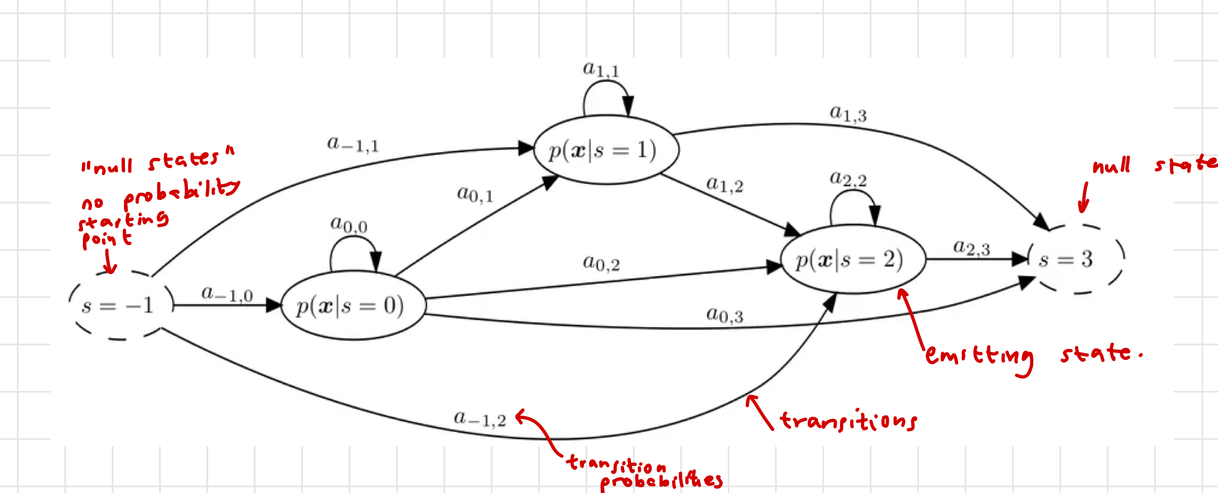
We do not know which state is active at any given time. This is why we refer to the model as a hidden Markov model, the states are hidden from us.

$s_t$ is the state at time (sample) $t$. Since $s_0\in \{0,1,2\}$, the state at time zero can be any of the possible states. We add an known initialisation state (-1) and an end state (N). These states have no associated probability densities and are known as null states. The other states are called emitting states since they have associated densities which can be used to generate new feature vectors.

For this reason HMMs are generative models

Each emitting state behaves like a Naive Bayes system and has a distribution describing its feature vectors:

$$P({\mathbf{x}}_t|s_t=j)$$

This gives the probability of the observation being generated by a specific state. With:

• $t$ being the time instant ($0:T-1$)
• $j$ being the state number ($0:N-1$)

Transitions between states are also probabilistic and modelled by the state transition matrix $A$ with:

$$a_{i,j}=P(s_t=j|s_{t-1}=i)$$

Given the current state is $s=i$, then $a_{i,j}$ is the probability that the next feature vector is generated by $s=j$.

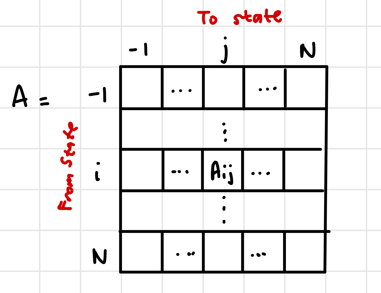
In Python, the transition matrix has a specific shape to reduce the memory used:

• The termination state N has no exiting states, and therefore may be omitted from the matrix to produce a N+1 row matrix.
• Since Python interprets negative indexes as counting backwards from the array, the -1 index is actually located at the Nth index.
• We can omit the -1 (last column) from the matrix since the initial state has no entering states.

This results in a N + 1 by N + 1 matrix, with rows $0,\dots ,N-1,-1$ and columns $0,\dots ,N$

Fundamental Assumptions

HMMs make two important assumptions about the relationship between the feature vectors:

1. Observation Independence

$$P({\mathbf{x}}_t|{\mathbf{x}}_{0:t-1},s_{-1,t})=P({\mathbf{x}}_t|s_t)$$

Given we know all the observations before the current feature vector and all states up till the current time, the likelihood of the $t$-th feature vector is only dependant on the current state $s_t$ and is unaffected by both the previous states and feature vector sequence.

2. First Order Markov

$$P(s_t|{\mathbf{x}}_{0:t},s_{-1,t-1})=P(s_t|s_{t-1})$$

The probability distribution of the current state, given both prior states and observations, is only dependant on the previous state.

HMM Topologies

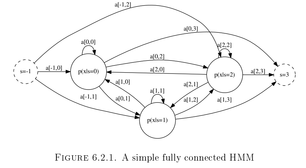
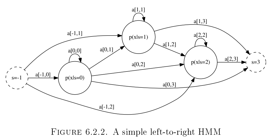
How does one choose the topology to use?

Bayesian techniques allow us to learn/infer the structure to choose the topology. We will not focus on that method in this course.

Instead, one can use prior knowledge to choose the topology:

• Left to right models are used when we have signals with a very definite time order which is non-repeating.
• Fully connected models are used for long repetitive sequence modelling.

Calculating the Likelihoods

We’d like to match a sequence of feature vectors to a model and get a likelihood score.

$$P({\mathbf{x}}_{0:T-1}|M)$$

The likelihood of sequence being generated by model $M$.

The Statistics

1. Product Rule: $P(a,b|c)=P(a|b,c)P(b|c)$ or $P(a,b)=P(a|b)P(b)$
2. Sum Rule: $P(a)={\sum }_{i}P(a,b_i)$
3. Observation Independence: $P({\mathbf{x}}_t|{\mathbf{x}}_{0:t-1},s_{-1,t})=P({\mathbf{x}}_t|s_t)$
4. First Order Markov: $P(s_t|{\mathbf{x}}_{0:t},s_{-1,t-1})=P(s_t|s_{t-1})$

Direct Approach

We can solve the likelihood using marginalisation of all possible state sequence likelihoods:

$$P({\mathbf{x}}_{0:T-1})=\sum _{\forall s_{-1:T}}P({\mathbf{x}}_{0:T-1},s_{-1:T})$$

Notice that the given $M$ is implicit ($P({\mathbf{x}}_{0:T-1}|M))$

We can solve for the joint probability as follows:

$$\begin{array}{rl}& P({\mathbf{x}}_{0:T-1},s_{-1:T})\\ =& P(s_T|{\mathbf{x}}_{0:T-1},s_{-1:T-1})P({\mathbf{x}}_{0:T-1},s_{-1:T-1})\text{ (product rule)}\\ =& P(s_T|s_{T-1})P({\mathbf{x}}_{0:T-1},s_{-1:T-1})\text{ (first order markov)}\\ =& a_{s_{T-1},s_T}P({\mathbf{x}}_{0:T-1},s_{-1:T-1})\\ =& a_{s_{T-1},s_T}P({\mathbf{x}}_{T-1}|{\mathbf{x}}_{0:T-2},s_{-1:T-1})P({\mathbf{x}}_{0:T-2},s_{-1:T-1})\text{ (product rule)}\\ =& a_{s_{T-1},s_T}P({\mathbf{x}}_{T-1}|s_{T-1})P({\mathbf{x}}_{0:T-2},s_{-1:T-1})\text{ (observation independence)}\end{array}$$

From this, we can see the last term is of the same form as the original probability, but one timestep shorter. Therefore we can solve for this likelihood recursively:

$$P({\mathbf{x}}_{0:T-1},s_{-1:T})=a_{s_{T-1},s_T}P({\mathbf{x}}_{T-1}|s_{T-1})a_{s_{T-2},s_{T-1}}P({\mathbf{x}}_{T-2}|s_{T-2})\dots a_{-1,s_0}$$

All these values are known or can be easily calculated. Thus, we have found a solution to the likelihood.

This approach in prohibitively complex to calculate due to the sum over all possible state sequences. The algorithm is $O(N^T)$ complex as the possible state sequences grow exponentially with the length of the sequence.

This approach, however, does provide insights and fundamental understanding to how the sequences are calculated.

The highest scoring sequence is the optimal sequence

Forward Algorithm

We need an algorithm that can efficiently calculate the likelihoods in an efficient manner.

We define a new term, which we’ll called the forward likelihood:

$${\alpha }_t(j)\triangleq P({\mathbf{x}}_{0:t},s_t=j)$$

Again, we want to find a recursive solution to this likelihood function:

$$\begin{array}{rl}{\alpha }_t(j)& =P({\mathbf{x}}_{0:t},s_t=j),\text{ for }t=1:T-1\text{ and }j=0:N-1\\ & =P({\mathbf{x}}_t|{\mathbf{x}}_{0:t-1},s_t=j)P({\mathbf{x}}_{0:t-1},s_t=j)\text{ (product rule)}\\ & =P({\mathbf{x}}_t|s_t=j)P({\mathbf{x}}_{0:t-1},s_t=j)\text{ (observation independence)}\\ & \text{next we split out the prior state into a sum}\\ & =P({\mathbf{x}}_t|s_t=j)\sum _{i=0}^{N-1}P({\mathbf{x}}_{0:t-1},s_{t-1}=i,s_t=j)\text{ (sum rule)}\\ & =P({\mathbf{x}}_t|s_t=j)\sum _{i=0}^{N-1}P(s_t=j|{\mathbf{x}}_{0:T-1},s_{t-1}=i)P({\mathbf{x}}_{0:t-1},s_{t-1}=i)\text{ (product rule)}\\ & =P({\mathbf{x}}_t|s_t=j)\sum _{i=0}^{N-1}P(s_t=j|,s_{t-1}=i)P({\mathbf{x}}_{0:t-1},s_{t-1}=i)\text{ (first order markov)}\\ & =P({\mathbf{x}}_t|s_t=j)\sum _{i=0}^{N-1}{a}_{i,j}P({\mathbf{x}}_{0:t-1},s_{t-1}=i)\end{array}$$

Once again, the final term is the same as the original but one timestep less. We can recurse once more.

$${\alpha }_t(j)=P({\mathbf{x}}_t|s_t=j)\sum _{i=0}^{N-1}{a}_{i,j}\cdot {\alpha }_{t-1}(i),\text{ for }t=1:T-1\text{ and }j=0:N-1$$

For the initialisation:

$${\alpha }_{-1}(j)=\{\begin{array}{ll}1& \text{with }j=-1\\ 0& \text{otherwise}\end{array}$$

and

$${\alpha }_0(j)=P({\mathbf{x}}_0|s_0=j)\sum _{i=0}^{N-1}{a}_{i,j}\cdot {\alpha }_{-1}(i)=P({\mathbf{x}}_0|s_0=j)a_{-1,j}$$

We then use the forward likelihood to calculate the total likelihood:

$$\begin{array}{rl}P({\mathbf{x}}_{0:T})& =\sum _{j=0}^{N-1}P({\mathbf{x}}_{0:T-1},s_{T-1}=j,s_T=N)\\ & =\sum _{j=0}^{N-1}P(s_T=N|{\mathbf{x}}_{0:T-1},s_{T-1}=j)P({\mathbf{x}}_{0:T-1},s_{T-1}=j)\text{ (product rule)}\\ & =\sum _{j=0}^{N-1}P(s_T=N|s_{T-1}=j)P({\mathbf{x}}_{0:T-1},s_{T-1}=j)\text{ (first order markov)}\\ & =\sum _{j=0}^{N-1}{a}_{j,N}\cdot {\alpha }_{T-1}(j)\end{array}$$

Final state $s_T$ is the terminating state $N$.

This algorithm is $O(N^{2}T)$ in time complexity. Much more manageable.

We pack ${\alpha }_t(j)$ into a matrix.

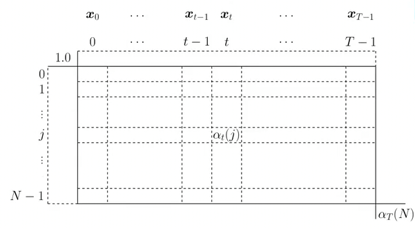
We fill it as follows:

1. First column: ${\alpha }_{-1}(-1)=1$
2. Second column: ${\alpha }_0(j)=P({\mathbf{x}}_0|s_0=j)a_{-1,j}$
3. Recursively fill columns: ${\alpha }_t(j)=P({\mathbf{x}}_t|s_t=j){\sum }_{i=0}^{N-1}{a}_{i,j}\cdot {\alpha }_{t-1}(i)$
4. Final column: ${\alpha }_T(N)={\sum }_{j=0}^{N-1}{a}_{j,N}\cdot {\alpha }_{T-1}(j)$

Therefore the final algorithm is:

1. Filling the matrix as above
2. Computing the likelihoods: $P({\mathbf{x}}_{0:T})={\sum }_{j=0}^{N-1}{a}_{j,N}\cdot {\alpha }_{T-1}(j)$

Numerical Stability

During the recursive calculation, the numbers grow exceedingly small, resulting in underflow. To solve this we should use log scale.

$$\begin{array}{rl}\log ({\alpha }_t(j))& =\log (P({\mathbf{x}}_t|s_t=j))+\log (\sum _i{a}_{i,j}\cdot {\alpha }_{t-1}(i))\end{array}$$

We can still have underflow in the second term with the summation. To combat this we’ll use the log-sum exponent trick

$$\begin{array}{rl}L& =\log (\sum _i{e}^{L_i}),\text{ with }{L}_i=a_{i,j}\cdot {\alpha }_{t-1}(i)\\ L& =\log (e^{L_M}(e^{L_0-L_M}+e^{L_1-L_M}+\dots +e^0+\dots +e^{L_{N-1}-L_M}))\\ & =L_M+\log (\sum _i{e}^{L_i-L_M})\\ & \text{ with }{L}_M=\underset{i}{\max }{L}_i\end{array}$$

Viterbi Algorithm: Most Likely State Sequence Calculation

$${\delta }_t(j)\triangleq \underset{s_{-1}:t_{-1}}{\max }P({\mathbf{x}}_{0:t},s_{-1,t-1},s_t=j)$$

TODO: show derivation to the simplification below

We’re essentially replacing the summation in the forward algorithm with maximisation.

$${\delta }_t(j)=P({\mathbf{x}}_t|s_t=j)\underset{i=0:N-1}{\max }{a}_{i,j}\cdot {\delta }_{t-1}(i)$$

We also keep track of the index which produced the maximum value, we call this the back pointer:

$$b_t(j)=\underset{i=0:N-1}{\mathrm{argmax}}{a}_{i,j}\cdot {\delta }_{t-1}(i)$$

Numerical Stability

Unlike the forward algorithm, taking the log does not require the log-sum exponent trick:

$$\log {\delta }_t(j)=\log P({\mathbf{x}}_t|s_t=j)+\log (\underset{i=0:N-1}{\max }{a}_{i,j}\cdot {\delta }_{t-1}(i))$$

Training

We’re to train the parameters of the HMM:

1. Transition Matrix
2. State distributions

For training we use $M$ training sequences. Training sequences need not be the same length.

M-Step

Suppose we know the state sequence associated with the training sequence of feature vectors. We could use the vectors beloning to each state to re-estimate the state distribution of all the states. Likewise, we can re-estimate the transition matrix by simply counting the number of transition and normalising it. See the equation below:

$${\hat{a}}_{i.j}=\frac{\#(s_t=i,s_{t+1}=j)}{\#(s_t=i)}$$

With $\#$ being a count of the occurrences in the argument.

Unfortunately, we do not know which feature vectors in the sequence map to which state, as per the underlying assumption of HMMs. However, estimating the HMM parameters, we can use the Viterbi algorithm to estimate the optimal state sequence for each observation, which can be used instead of the true sequences. Using expectation maximisation we can iteratively improve our estimate of the model parameters.

EM Algorithm: Viterbi Re-estimation

1. Initialisation: Get an initial HMM parameter set
   • Assign sensible state sequences to the training sequences
     • For a left-to-right model, one would typically subdivide the sequence into $N$ equal subsequences and assign each to the next state.
     • For fully-connected model, one might use clustering (GMM), this will provide both states for each observation and the state distributions.
   • Use the initial sequences to generate an initial model using the M-step
2. EM Re-estimation:
   1. Expectation: Determine the optimal state sequence for each training sequence, and calculate the log likelihood $\log P({\mathbf{x}}_{0:T-1},S^{\ast })$ - with $S^{\ast }$ being the viterbi estimated state sequence. Accumulate these ‘scores’ to test for convergence later: $f={\sum }_{\forall \text{ training }{\mathbf{x}}_{0:T-1}}\log P({\mathbf{x}}_{0:T-1},S^{\ast })$
   2. Maximisation: Perform the M-Step above to update the HMM parameters.
3. Termination: Compare the current and prior total score $f$. If it is in acceptable tolerance, terminate. Otherwise, repeat the EM Re-estimation step.

EM Algorithm: Baum Welch Re-estimation

The Viterbi Re-estimation method segments feature vectors into the particular state associated with each vector, it is a hard allocation (like KMeans).

Baum Welch’s Re-estimation performs soft allocation to each state (similar to how GMM assigns responsibility)

XXX: I’m not writing LaTeX for these formulas, so just go check the course notes

XXX: Let’s assume this section is not that important